Is it crowded in here? -

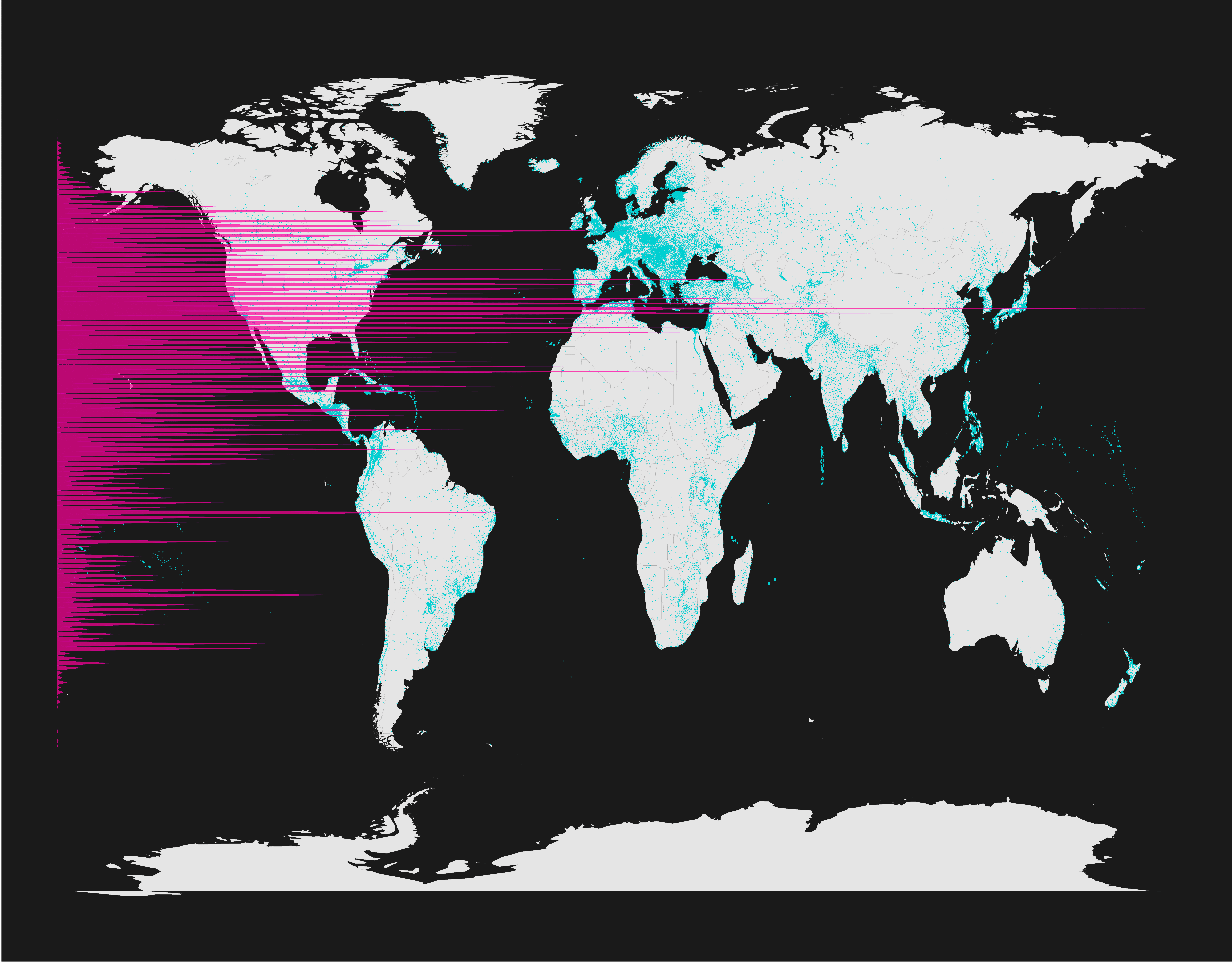
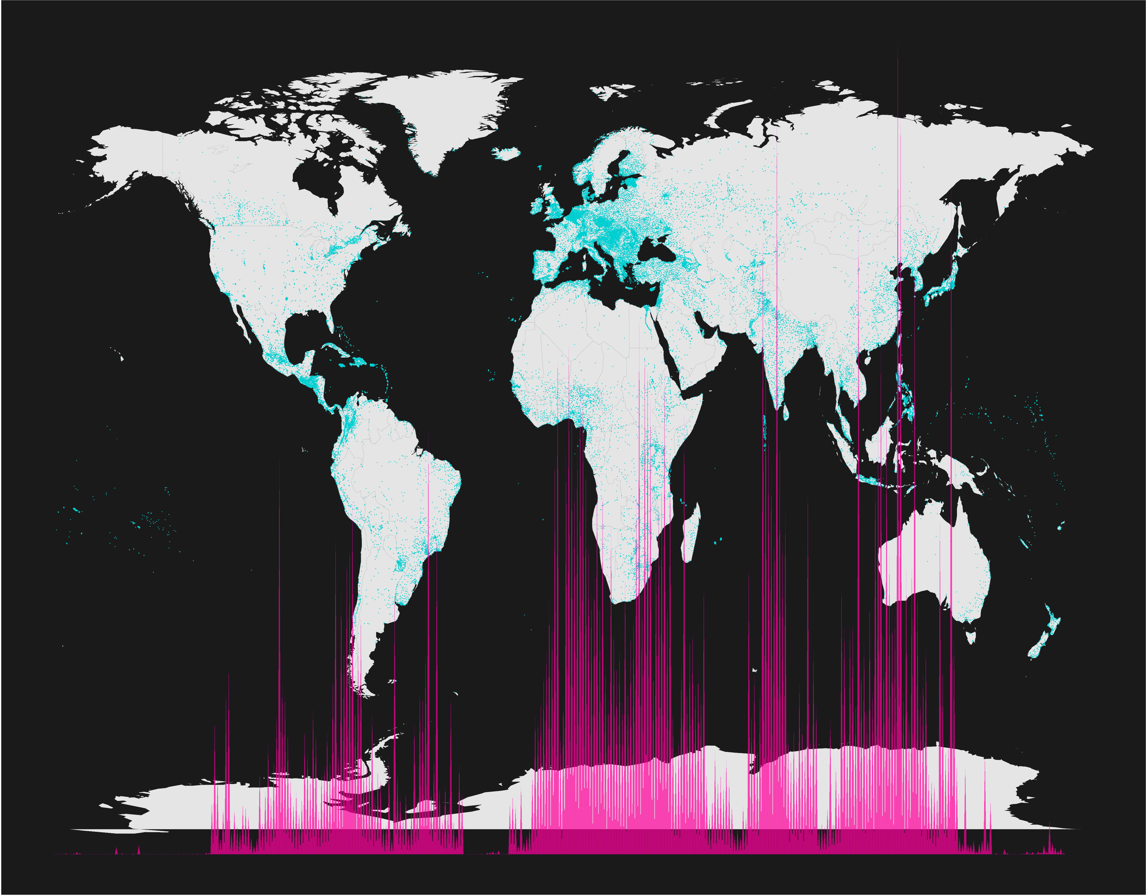
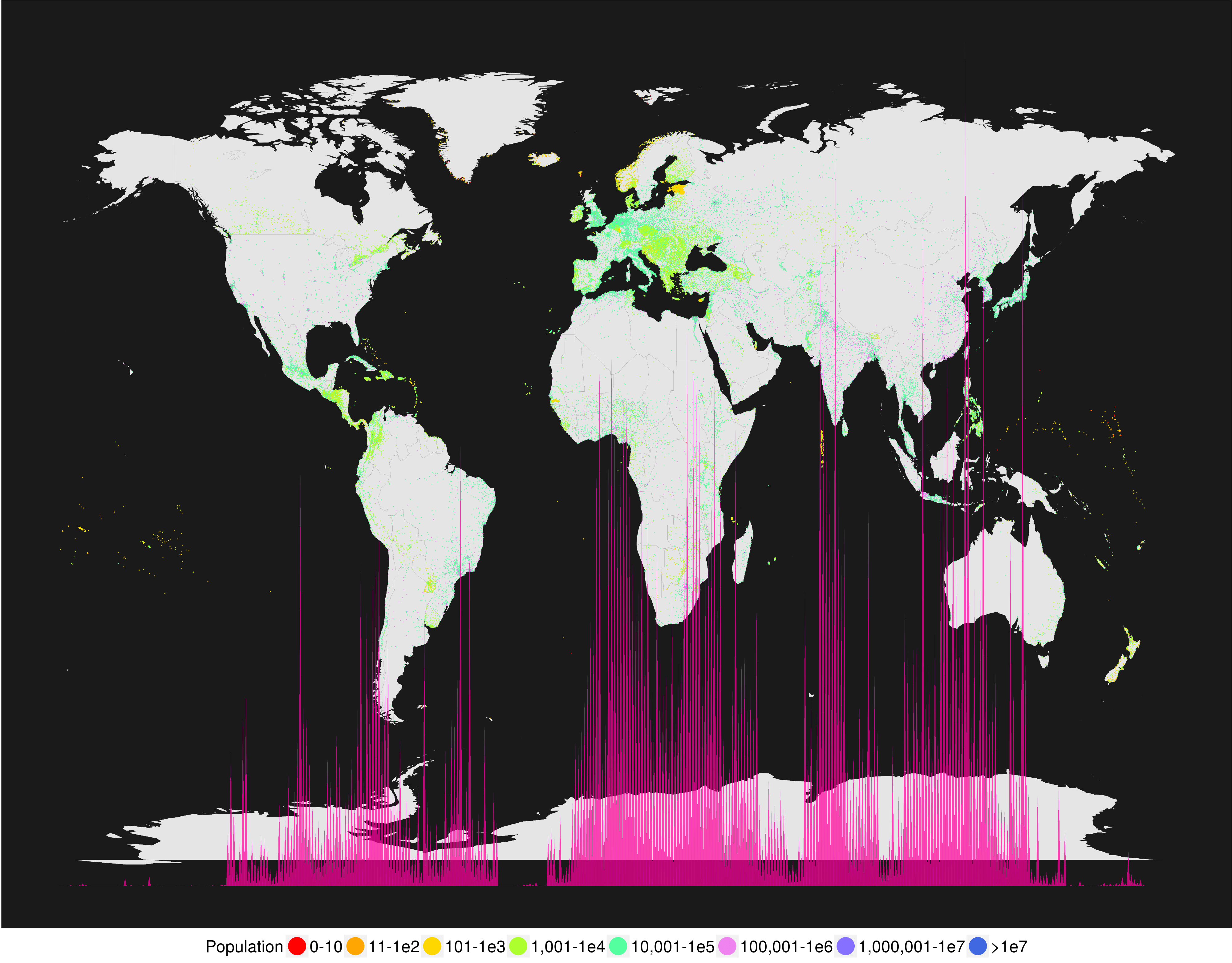
This was a neat graphic that someone made (i.imgur.com). It shows the population at a given latitude or longitude as a bar chart, overlayed on a map of the world itself. It shows where people live; the bigger the bar, the more people living at that latitude/longitude.

“I can do that.” I said. In R of course. So here it is;

	## libraries used to create these maps
	library(maps) ## world.cities data
	library(dplyr) ## group_by(), summarise(), and imported %>%
	library(ggplot2) ## plotting

	## the raw data
	## `citation("maps")`
	data("world.cities")

	## limit the data to the latitude, lonitude, and population
	XY <- world.cities %>% select(lat, long, pop) %>% rename(lon=long)

	## bin the lat/lon into 1 degree bins
	XY$binlat <- as.numeric(as.character(cut(XY$lat, breaks=seq(-90,90,1), labels=seq(-90,89,1))))
	XY$binlon <- as.numeric(as.character(cut(XY$lon, breaks=seq(-180,180,1), labels=seq(-180,179,1))))

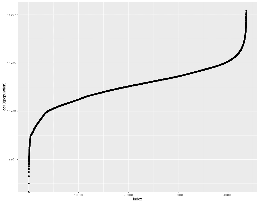
	## bin the population. What size bins?
	XY %>% arrange(pop) %>% ggplot(aes(x=1:nrow(.), y=pop)) + geom_point() + scale_y_log10() + xlab("Index") + ylab("log10(population)")
	## looks like powers of 10 will be good breaks
	XY$binpop <- cut(XY$pop, breaks=c(-1, 1e1, 1e2, 1e3, 1e4, 1e5, 1e6, 1e7, 1e10),
	labels=c("0-10", "11-1e2", "101-1e3", "1,001-1e4", "10,001-1e5", "100,001-1e6", "1,000,001-1e7", ">1e7"))

	## aggregate the population to the 1 degree bins
	XYmergeLat <- XY %>% group_by(binlat) %>% summarise(pop=sum(pop))
	XYmergeLon <- XY %>% group_by(binlon) %>% summarise(pop=sum(pop))

	## scale the population to the full range of lat/lon and shift to a zero scale
	XYmergeLat$pop <- ((XYmergeLat$pop/max(XYmergeLat$pop))*360L)-180
	XYmergeLon$pop <- ((XYmergeLon$pop/max(XYmergeLon$pop))*180L)-90

	## move the values to the centre of the bins
	XYmergeLat$binlat <- XYmergeLat$binlat + 0.5
	XYmergeLon$binlon <- XYmergeLon$binlon + 0.5

	## merge back with a data.frame of empty populations at the integer degree marks
	XYmergeLat <- merge(XYmergeLat, data.frame(binlat=seq(-90,90,1), pop=-180), all=TRUE)
	XYmergeLon <- merge(XYmergeLon, data.frame(binlon=seq(-180,180,1), pop=-90), all=TRUE)

	## plot the population-by-longitude data using ggplot2
	popByLon <- ggplot(XY) +
	## plot the world map polygons
	geom_polygon(aes_(~long, ~lat, group=~group), size=0.1, data=map_data("world", regions="."),
	fill="grey90", colour="grey50", inherit.aes=FALSE) +
	## plot the cities
	geom_point(aes(x=lon, y=lat, color=factor(binpop)), size=0.4) +
	## plot the population graph on the x-axis
	geom_polygon(data=XYmergeLon, aes(x=binlon, y=pop), colour=rgb(1,0,1,alpha=0.9),
	fill=rgb(1,0,0.6, alpha=0.7), size=0.05) +
	## clean up and remove unneccesary elements
	theme(panel.background=element_rect(fill="grey10", color="grey90"),
	line=element_blank(),
	axis.text=element_blank(),
	axis.title=element_blank(),
	legend.text=element_text(size=40),
	legend.title=element_text(size=40),
	plot.margin=unit(c(0,0,0,0), "lines"),
	complete=TRUE) +
	scale_color_manual(name="Population",
	values=c("0-10"="red",
	"11-1e2"="orange",
	"101-1e3"="gold",
	"1,001-1e4"="greenyellow",
	"10,001-1e5"="seagreen1",
	"100,001-1e6"="violet",
	"1,000,001-1e7"="lightslateblue",
	">1e7"="royalblue")) +
	theme(legend.position="bottom") +
	guides(color=guide_legend(nrow=1, override.aes=list(size=20)))

	## FORMAL: repeat for the population-by-latitude, except reverse lat and lon then coord_flip()
	## INFORMAL: is it worth it, let me work it. put my coords down, flip it, and reverse it
	popByLat <- ggplot(XY) +
	geom_polygon(aes_(~lat, ~long, group=~group), size=0.1, data=map_data("world", regions="."),
	fill="grey90", colour="grey50", inherit.aes=FALSE) +
	## plot the cities
	geom_point(aes(x=lat, y=lon, color=factor(binpop)), size=0.4) +
	geom_polygon(data=XYmergeLat, aes(x=binlat, y=pop), colour=rgb(1,0,1,alpha=0.9),
	fill=rgb(1,0,0.6, alpha=0.7), size=0.05) + coord_flip() +
	theme(panel.background=element_rect(fill="grey10", color="grey90"),
	line=element_blank(),
	axis.text=element_blank(),
	axis.title=element_blank(),
	legend.text=element_text(size=40),
	legend.title=element_text(size=40),
	plot.margin=unit(c(0,0,0,0), "lines"),
	complete=TRUE) +
	scale_color_manual(name="Population",
	values=c("0-10"="red",
	"11-1e2"="orange",
	"101-1e3"="gold",
	"1,001-1e4"="greenyellow",
	"10,001-1e5"="seagreen1",
	"100,001-1e6"="violet",
	"1,000,001-1e7"="lightslateblue",
	">1e7"="royalblue")) +
	theme(legend.position="bottom") +
	guides(color=guide_legend(nrow=1, override.aes=list(size=20)))

	## show the plots
	popByLon
	popByLat

view raw (gist.github.com) population.R (gist.github.com) hosted with ❤ by GitHub (github.com)

I love that such a small amount of code can produce something so interesting. Click the images below to view them in all their full-size glory.

How is this useful? Well… okay, it’s not. It’s pretty. That’s what it is. An a neat exercise in data manipulation and plotting.

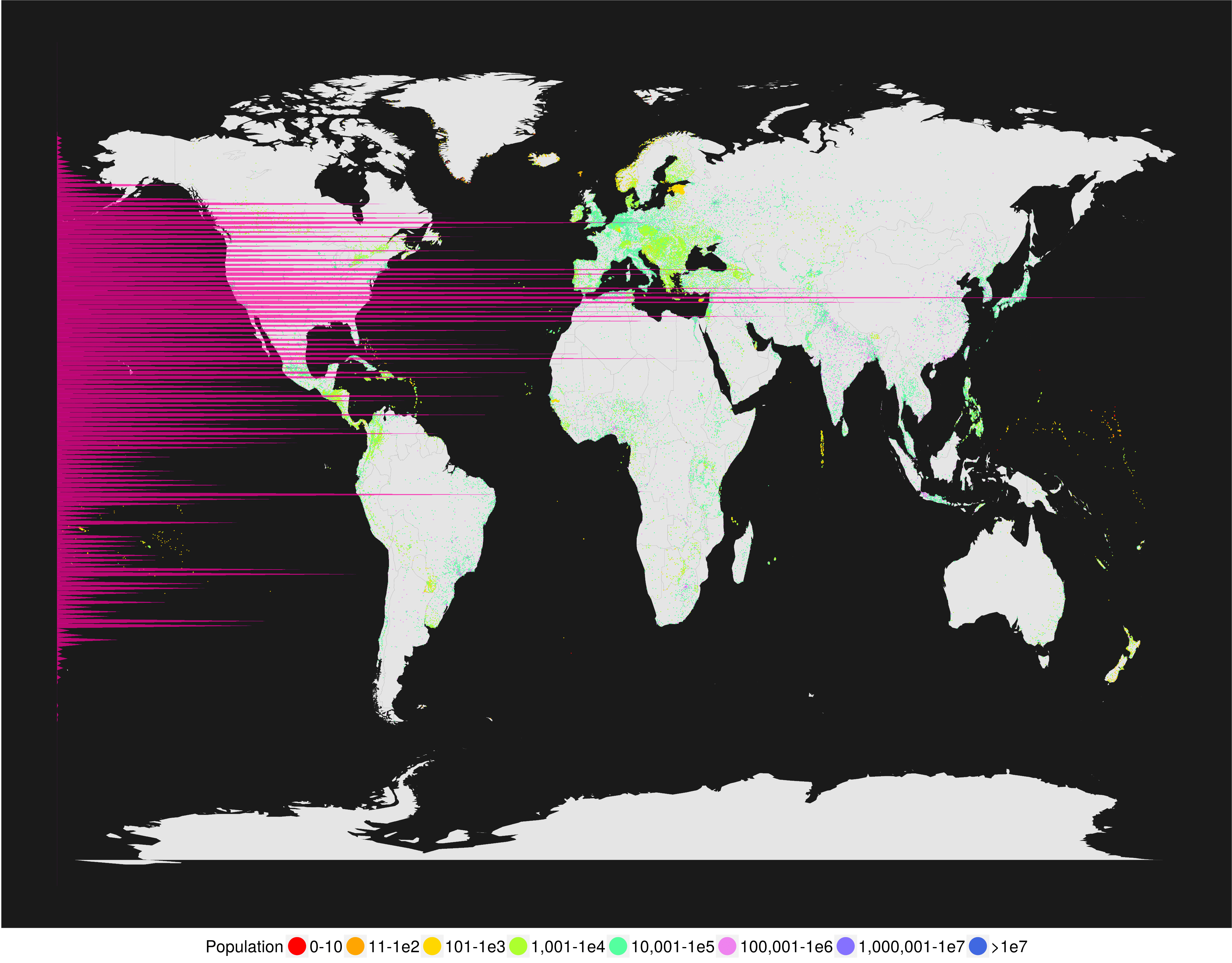
UPDATE: As per a comment on my reddit thread, I’ve updated this to include a logarithmic colour-scale for population. The populations follow a nice logit curve if you arrange them in order:

Here’s the updated graphics:

rstats

See also