Data Munging With R Preview - Storing Values (Assigning)

[Update] The title of this book has since been changed to Beyond Spreadsheets with R.

Since about October last year, I’ve been writing an introduction to R book. It’s been quite the experience. I’ve finally started making time to document some of the interesting things I’ve learned (about R, about writing, about how to bring those two together) along the way.

The book is aimed at proper beginners; people with absolutely no formal coding experience. This tends to mean people coming from Excel who need to do more than a spreadsheet can/should.

I'm writing an R book for real beginners (ppl with 0 code XP) via @ManningBooks! What tripped you up most when you first learned R? Pls RT!

— Jonathan Carroll (@carroll_jono) September 27, 2016

Most of the books I’ve looked at which claim to teach programming begin with some strong assumptions about the reader already knowing how to program, and teach the specific syntax of some language. That’s no good if this is your first language, so I’m working towards teaching the concepts, the language, and the syntax (warts and all).

The book is currently available under the Manning Early Access Program (MEAP) which means if you buy it you get the draft of the first three chapters right now. If you find something you still don’t understand, or you don’t like how I’ve written some/all of it, then jump onto the forum and let me know. I make more edits and write more chapters, and you get updated versions. Lather, rinse, repeat until the final version and you get a polished book which (if I’m any good) contains what you want it to.

I’m genuinely interested in getting this right; I want to help people learn R. I contribute a bit of time on Stack Overflow answering people’s questions, and it’s very common to see questions that shouldn’t need asking. I don’t blame the user for not knowing something (a different answer for not searching, perhaps), but I can help make the resource they need.

To show that I really want people to contribute, here’s a discount code to sweeten the deal: use mlcarroll for 50% off here.

Chapter 1 is a free download, so please check that out too! At the moment the MEAP covers the first three chapters, but the following four aren’t too far behind.

I’ll document some of the behind-the-scenes process shortly, but for now here’s an excerpt from chapter 2:

2.2. Storing Values (Assigning)

In order to do something with our data, we will need to tell R what to call it, so that we can refer to it in our code. In programming in general, we typically have variables (things that may vary) and values (our data). We’ve already seen that different data values can have different types, but we haven’t told R to store any of them yet. Next, we’ll create some variables to store our data values.

2.2.1. Data (Variables)

If we have the values 4 and 8 and we want to do something with them, we can use the values literally (say, add them together as 4 + 8). You may be familiar with this if you frequently use Excel; data values are stored in cells (groups of which you can opt to name) and you tell the program which values you wish to combine in some calculation by selecting the cells with the mouse or keyboard. Alternatively, you can opt to refer to cells by their grid reference (e.g. A1). Similarly to this second method, we can store values in variables (things that may vary) and abstract away the values. In R, assigning of values to variables takes the following form

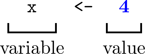
variable <- value

The assignment operator <- can be thought of as storing the value/thing on the right hand side into the name/thing on the left hand side. For example, try typing x <- 4 into the R **Console** then press Enter:

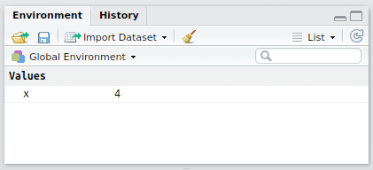
Figure 2. 1. The variable x has been assigned the value 4. You could just as easily use the equals sign to achieve this; x = 4 but I recommend you use <- for this for reasons that will become clear later. You’ll notice that the **Environment** tab of the **Workspace** pane now lists x under **Values** and shows the number 4 next to it, as shown in Fig 2. 2.

Figure 2. 2. The variable x has been assigned the value 4.

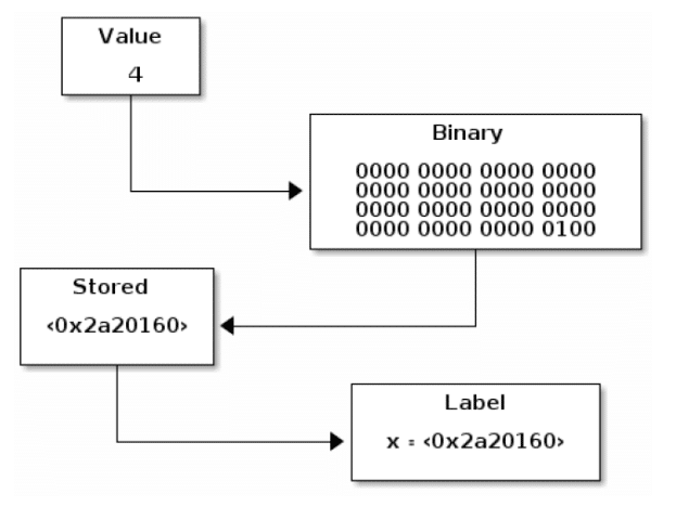
What happened behind the scenes was that when we pressed Enter, R took the entire expression that we entered (x <- 4) and evaluated it. Since we told R to assign the value 4 to the variable x, R converted the value 4 to binary and placed that in the computer’s memory. R then gives us a reference to that place in the computer’s memory and labels it x. A diagram of this process is shown in Fig 2. 3. Nothing else appeared in the **Console** because the action of assigning a value doesn’t return anything (we’ll cover this more in our section on functions).

Figure 2. 3. Assigning a value to a variable. The value entered is converted to binary, then stored in memory, the reference to which is labelled by the variable.

This is overly simplified, of course. Technically speaking, in R, names have objects rather than the other way around. This means that R can be quite memory efficient since it doesn’t create a copy of anything it doesn’t need to.

Caution: On “hidden” variables

Variables which begin with a period (e.g. .length) are considered hidden and do not appear in the **Environment** tab of the **Workspace**. They otherwise behave exactly as any other variable; they can be printed and manipulated. An example of one of these is the .Last.value variable, which exists from the moment you load up R (with the value TRUE) - this contains the output value of the last statement executed (handy if you forgot to assign it to something). There are very few reasons you’ll want to use this feature (dot-prefixed hidden variables) on purpose at the moment, so for now, avoid creating variable names with this pattern. The exception to the hidden nature of these is again the .Last.value variable which you can request to be visible in the **Environment** tab via Tools ▸ Global Options…  ▸ General ▸ Show .Last.value in environment listing.

We can retrieve the value assigned to the variable x by asking R to print the value of x

print(x = x)

## [1] 4

for which we have a useful shortcut - if your entire expression is just a variable, R will assume you mean to print() it, so

x

## [1] 4

works just the same.

Now, about that [1]: it’s important to know that in R, there’s no such thing as a single value; every value is actually a vector of values (we’ll cover these properly in the next chapter, but think of these as collections of values of the same type).^[1]

Whenever R prints a value it allows for the case where the value contains more than one number. To make this easier on the eye, it labels the first value appearing on the line by it’s position in the collection. For collections (vectors) with just a single value, this might appear strange, but this makes more sense once our variables contain more values

# Print the column names of the mtcars dataset
names(x = mtcars)

##  [1] "mpg"  "cyl"  "disp" "hp"   "drat" "wt"   "qsec" "vs"   "am"   "gear"
## [11] "carb"

We can assign another variable to another value

y <- 8

There are few restrictions for what we can name our data values, but R will complain if you try to break them. Variables should start with a letter, not a number. Trying to create the variable 2b will generate an error. Variables can also start with a dot (.) as long as it’s not immediately followed by a number, although you may wish to avoid doing so. The rest of the variable name can consist of letters (upper and lower case) and numbers, but not punctuation (except . or _) or other symbols (except the dot, though again, preferably not).

There are also certain reserved words that you can’t name variables as. Some are reserved for built-in functions or keywords

if, else, repeat, while, function, for, in, next, and break.

Others are reserved for particular values

TRUE, FALSE, NULL, Inf, NaN, NA, NA_integer_, NA_real_, NA_complex_, and NA_character_.

We’ll come back to what each of these means, but for now you just need to know that you can’t create a variable with one of those names.

Caution: On overwriting names

What you can do however, which you may wish to take care with, is overwrite the in-built names of variables and functions. By default, the value pi is available (π = 3.141593).

If you were translating an equation into code, and wanted to enter the value p_i you might accidentally call it pi and in doing so change the default value, causing all sorts of trouble when you next go to use it or call a function you’ve written which expects it to still be the default.

The default value can still be accessed by specifying the package in which it is defined, separated by two colons (::). In the case of pi, this is the base package.

# Re-defining `pi` to be equal to exactly `3`
pi <- 3L
# The default, correct value is still available.
base::pi

## [1] 3.141593

This is also an issue for functions, with the same solution; specify the package in which it is defined to use that definition. We’ll return to this in a section on ‘scope’.

We’ll cover how to do things to our variables in more detail in the next section, but for now let’s see what happens if we add our variables x and y in the same way as we did for our regular numbers

x + y

## [1] 12

which is what we got when we added these numbers explicitly. Note that since our expression produces just a number (no assignment), the value is printed. We’ll cover how to add and subtract values in more depth in our section on basic mathematics.

R has no problems with overwriting these values, and it doesn’t mind what data you overwrite these with.^[2]

y <- 'banana'
y

## [1] "banana"

R is case-sensitive, which means that it treats a and A as distinct names. You can have a variable named myVariable and another named MYvariable and another named myVARIABLE and R will hold the value assigned to each independently.

On variable names:

There are only two hard things in Computer Science: cache invalidation and naming things.

a <- 4
b <- 8
sum_of_a_and_b <- a + b

print(x = sum_of_a_and_b)

## [1] 12

b <- 2

print(x = sum_of_a_and_b)

## [1] 12

str(object = mtcars, indent.str = '>>  ')

## 'data.frame':    32 obs. of  11 variables:
## >>  $ mpg : num  21 21 22.8 21.4 18.7 18.1 14.3 24.4 22.8 19.2 ...
## >>  $ cyl : num  6 6 4 6 8 6 8 4 4 6 ...
## >>  $ disp: num  160 160 108 258 360 ...
## >>  $ hp  : num  110 110 93 110 175 105 245 62 95 123 ...
## >>  $ drat: num  3.9 3.9 3.85 3.08 3.15 2.76 3.21 3.69 3.92 3.92 ...
## >>  $ wt  : num  2.62 2.88 2.32 3.21 3.44 ...
## >>  $ qsec: num  16.5 17 18.6 19.4 17 ...
## >>  $ vs  : num  0 0 1 1 0 1 0 1 1 1 ...
## >>  $ am  : num  1 1 1 0 0 0 0 0 0 0 ...
## >>  $ gear: num  4 4 4 3 3 3 3 4 4 4 ...
## >>  $ carb: num  4 4 1 1 2 1 4 2 2 4 ...

score <- 4.8
score

## [1] 4.8

str(object = score)

##  num 4.8

fruit <- 'banana'
fruit

## [1] "banana"

str(object = fruit)

##  chr "banana"

first_name <- 'John'
last_name  <- 'Smith'
top_points <- 23

a <- 3

a < - 3

## [1] FALSE