Another day, another compulsion to see if I can do any better than someone’s solution.
This one also comes from the FiveThiryEight Puzzler challenge courtesy of Xi’an
The original challenge this time was
The misanthropes are coming. Suppose there is a row of some number, N, of houses in a new, initially empty development. Misanthropes are moving into the development one at a time and selecting a house at random from those that have nobody in them and nobody living next door. They keep on coming until no acceptable houses remain. At most, one out of two houses will be occupied; at least one out of three houses will be. But what’s the expected fraction of occupied houses as the development gets larger, that is, as N goes to infinity?
which seems straightforward enough. Xi’an has a nice writeup of the analytical solution (which looks pretty well thought out) but that’s not what caught my attention. The (probably not intentionally provocative) statements
A riddle from The Riddler where brute-force simulation does not pay:
Hence this limits the realisation of simulation to, say, N=104
however, are like a red flag to a bull for me. The code provided for Xi’an’s solution isn’t optimised, and doesn’t take advantage of some potential speed-ups. 10,000 iterations seems like it should be quick. There’s also a typo in the microbenchmark code there; time should be times otherwise it’s passed as a lambda function evaluating time=10. Anyway, improvements to the code can be made.
I took a slightly different approach; I assigned a vector of ‘houses’ being either occupied or available, identified as such by a boolean (TRUE/FALSE). For the purposes of this question, available means that there is a) no occupant; b) no occupant on either side. The function I ended up with was
misanthropist <- function(N) {

  occupied   <- rep(FALSE, N)
  acceptable <- rep(TRUE, N)

  while(any(acceptable)) {
    possible <- .Internal(which(acceptable))
    occupied[movedin <- possible[.Internal(sample(length(possible), 1, FALSE, NULL))]] <- TRUE
    acceptable[c(movedin-1, movedin, movedin+1)] <- FALSE
  }

  return(mean(occupied))
}

library(compiler)
misanthropist_c <- cmpfun(misanthropist)
There are a heap of tricks employed here to speed evaluation up, and a few that aren’t because it turns out they didn’t perform better.
-
the
acceptablevector is populated independently of theoccupiedvector;acceptable = ! occupiedseemed like it was a contender but ended up being slower. -
any(acceptable)works faster thansum(acceptable)>0in thewhileloop, presumably because of short-circuiting (we only need to know that one isTRUE, at which point we don’t need to keep testing). -
I’ve used
.Internalcalls where possible (which,sample); this removes a tiny bit of overhead. -
the switching of
acceptabletoFALSEfor the newly occupied house and those on either side can be done in a single step via ac()subsetting. Originally I had coded around the potential issues of trying to setacceptable[0]oracceptable[N+1]when their neighbours moved in, but as it turns out, R is happy to silently assign beyond the bounds of that vector and move on, so no more checks needed. -
the proportion of occupied houses is easily calculated at the end given that
as.integer(TRUE)==1andas.integer(FALSE)==0, so the mean of the boolean vector is the proportion ofTRUEvalues. -
finally, I’ve byte-compiled the function with
compiler::cmpfun. Built-in functions inbaseare already byte-compiled, and this helps just a little bit more.
Back to the original question; how many iterations can we do? First, let’s compare what we’ve got so far with a reasonable number of iterations
> microbenchmark(frqns(1000L), misanthropist_c(1000L), times=3, unit="ms")
Unit: milliseconds
                   expr         min          lq        mean      median          uq         max neval
           frqns(1000L) 3600.981381 3601.460353 3655.512618 3601.939325 3682.778237 3763.617149     3
 misanthropist_c(1000L)    3.447858    3.470277    3.512251    3.492697    3.544448    3.596199     3
Uh, yep. That’s, just a little bit faster. Smidgen. 3.5ms/1000 iterations. What about a few more iterations on my optimised function? How about that 10,000 limit?
> microbenchmark(misanthropist_c(10000L), times=3, unit="ms")
Unit: milliseconds
                    expr      min       lq     mean   median       uq      max neval
 misanthropist_c(10000L) 194.0501 194.8379 198.7545 195.6258 201.1066 206.5875     3
Maybe we shouldn’t get too cocky. 10 times as many iterations takes 56 times longer.
> microbenchmark(misanthropist_c(100000L), times=3, unit="ms")
Unit: milliseconds
                     expr      min       lq    mean  median       uq      max neval
 misanthropist_c(100000L) 18260.85 18355.87 18422.4 18450.9 18503.18 18555.47     3
That brings us up to 184ms/1000 iterations. 10 times as many iterations again takes 92 times longer. It’s definitely slowing down.

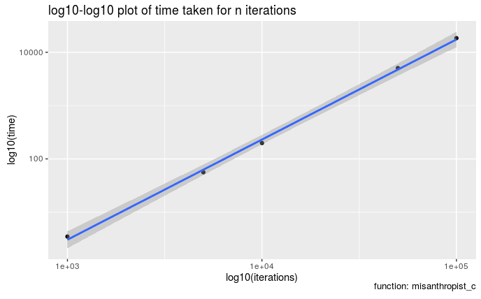
On a log-log plot of time against iterations with a slope of 2, it’s clearer that the problem scales as \(\mathcal{O}(n^2)\). That suggests that we should be able to complete the 1,000,000 iteration evaluation in about 20 minutes. 2,000,000 iterations in around 1 hour 20 minutes. 3,000,000 in 3 hours. Where am I going with this you ask? Xi’an requested help from stackexchange (a great move which paid off well) to get the analytical solution to the problem. If you check the timestamps, you’ll notice
# asked    Apr 25 at 14:04
# answered Apr 25 at 16:25
So, let’s say that stackexchange was offline when you were impatiently working on a solution, you coded perfectly and knew how to optimise your functions. How close to the right answer can you get in this amount of time (2.5 hours). We can probably do at most 2,000,000 iterations. Does that reach a close-enough solution? Rather than making my code run for that long, let’s see if Xi’an’s recursive equation gets the same answer (obviously faster).
xian <- function(N) {
  a=b=1
  for (n in 3:N){ C=(1+2*a+(n-1)*b)/n;a=b;b=C}
  return(C/N)
}

xian1e5 <- xian(1e5L)
mine1e5 <- misanthropist_c(1e5L)
format(2*100*(xian1e5 - mine1e5)/(xian1e5 + mine1e5), digits=3)
## [1] "-0.0335"so off by 0.07% at that stage, presumably getting closer with more iterations. Let’s use the recursive equation for this next bit then, knowing that in the above scenario we would be using the full iterative approach. The recursive expression itself can also be optimised. I did re-write it in C (xian_c) to see if that helped, but compiler:cmpfun (as xian_c2) does just as good a job (as one might expect)
> microbenchmark(xian(1e7), xian_c(1e7), xian_c2(1e7), times=5, unit="ms")
Unit: milliseconds
           expr        min         lq       mean     median         uq        max neval
 xian(1e+07)    16881.8007 16920.1492 16935.2306 16931.9014 16963.9973 16978.3044     5
 xian_c(1e+07)    114.8676   115.0287   115.0771   115.0948   115.1507   115.2438     5
 xian_c2(1e+07)   114.8645   114.9419   116.2547   114.9835   117.2379   119.2454     5
so clearly some improvements can be made. This one scales much better with iterations, to the point that I can just max it out
.Machine$integer.max
# 2147483647
format(xian_c(.Machine$integer.max), digits=20)
                  # 0.43233235833753796973
0.5*(1-exp(-2))   # 0.43233235838169364884
So now we have an upper limit on precision. We’ll be able to get at best within 0.0000000102% of the exact answer.
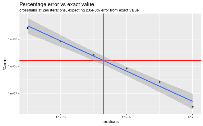
If I repeatedly use the xian_c function with different numbers of iterations, we can see how well we should expect to do

Is 2e-5% close enough for a couple of hours work?
And there we have it. If we’d been stuck with the non-recursive method and needed to get as close to the right answer as possible in a comparable time to obtaining the analytic solution and coding/running it, we could get pretty darn close. I’d say the brute-force method lives to see another day! … provided you do a bit of optimising and don’t mind worrying about the Halting problem.
Did I miss an important optimisation? Know a better approach? Hit the comments and let me know!
Title image © Copyright Jaggery and licensed for reuse under this Creative Commons Licence.
devtools::session_info()
## ─ Session info ──────────────────────────────────────────────────────────
##  setting  value
##  version  R version 3.5.2 (2018-12-20)
##  os       Pop!_OS 19.04
##  system   x86_64, linux-gnu
##  ui       X11
##  language en_AU:en
##  collate  en_AU.UTF-8
##  ctype    en_AU.UTF-8
##  tz       Australia/Adelaide
##  date     2019-08-13
##
## ─ Packages ──────────────────────────────────────────────────────────────
##  package     * version date       lib source
##  assertthat    0.2.1   2019-03-21 [1] CRAN (R 3.5.2)
##  backports     1.1.4   2019-04-10 [1] CRAN (R 3.5.2)
##  blogdown      0.14.1  2019-08-11 [1] Github (rstudio/blogdown@be4e91c)
##  bookdown      0.12    2019-07-11 [1] CRAN (R 3.5.2)
##  callr         3.3.1   2019-07-18 [1] CRAN (R 3.5.2)
##  cli           1.1.0   2019-03-19 [1] CRAN (R 3.5.2)
##  crayon        1.3.4   2017-09-16 [1] CRAN (R 3.5.1)
##  desc          1.2.0   2018-05-01 [1] CRAN (R 3.5.1)
##  devtools      2.1.0   2019-07-06 [1] CRAN (R 3.5.2)
##  digest        0.6.20  2019-07-04 [1] CRAN (R 3.5.2)
##  evaluate      0.14    2019-05-28 [1] CRAN (R 3.5.2)
##  fs            1.3.1   2019-05-06 [1] CRAN (R 3.5.2)
##  glue          1.3.1   2019-03-12 [1] CRAN (R 3.5.2)
##  htmltools     0.3.6   2017-04-28 [1] CRAN (R 3.5.1)
##  knitr         1.24    2019-08-08 [1] CRAN (R 3.5.2)
##  magrittr      1.5     2014-11-22 [1] CRAN (R 3.5.1)
##  memoise       1.1.0   2017-04-21 [1] CRAN (R 3.5.1)
##  pkgbuild      1.0.4   2019-08-05 [1] CRAN (R 3.5.2)
##  pkgload       1.0.2   2018-10-29 [1] CRAN (R 3.5.1)
##  prettyunits   1.0.2   2015-07-13 [1] CRAN (R 3.5.1)
##  processx      3.4.1   2019-07-18 [1] CRAN (R 3.5.2)
##  ps            1.3.0   2018-12-21 [1] CRAN (R 3.5.1)
##  R6            2.4.0   2019-02-14 [1] CRAN (R 3.5.1)
##  Rcpp          1.0.2   2019-07-25 [1] CRAN (R 3.5.2)
##  remotes       2.1.0   2019-06-24 [1] CRAN (R 3.5.2)
##  rlang         0.4.0   2019-06-25 [1] CRAN (R 3.5.2)
##  rmarkdown     1.14    2019-07-12 [1] CRAN (R 3.5.2)
##  rprojroot     1.3-2   2018-01-03 [1] CRAN (R 3.5.1)
##  sessioninfo   1.1.1   2018-11-05 [1] CRAN (R 3.5.1)
##  stringi       1.4.3   2019-03-12 [1] CRAN (R 3.5.2)
##  stringr       1.4.0   2019-02-10 [1] CRAN (R 3.5.1)
##  testthat      2.2.1   2019-07-25 [1] CRAN (R 3.5.2)
##  usethis       1.5.1   2019-07-04 [1] CRAN (R 3.5.2)
##  withr         2.1.2   2018-03-15 [1] CRAN (R 3.5.1)
##  xfun          0.8     2019-06-25 [1] CRAN (R 3.5.2)
##  yaml          2.2.0   2018-07-25 [1] CRAN (R 3.5.1)
##
## [1] /home/jono/R/x86_64-pc-linux-gnu-library/3.5
## [2] /usr/local/lib/R/site-library
## [3] /usr/lib/R/site-library
## [4] /usr/lib/R/library