Comparing R's {targets} and dbt for Data Engineering -

I’m getting more and more into data engineering these days and having used R for a long time, I’m seeing a lot of problems that look nail-shaped to my R-shaped hammer. The available tools to solve those problems exist for (presumably) very good reasons, so I wanted to take some time to dig into how to use them and compare their workflows to what I would otherwise naively do in R.

I should mention here that I’m currently open to data/code-related opportunities and am actively seeking a new role – if your organisation is looking for someone aligned with my skillset, please get in touch with me any way you can, e.g. contact at jcarroll.com.au.

I’m a firm believer in “you learn with your hands, not with your eyes” so I wanted to actually build something. I definitely could spin up Claude Code and have it produce the entire thing for me – and in a different project I might do that – but in this case I want to make the mistakes myself so I can learn where the complexity really lives and where my prior assumptions are misaligned. I did have Claude (the chat version, not the full coding agent) guide me through the steps to get this project running, and I did let it clean up my SQL; this project wasn’t about learning to better optimise my SQL, but understanding exactly what it produced will help me write a better version on my next iteration.

Thinking of a real-world project I could take for a spin, I decided to build some ingestion for my personal finances. I’ve used Quickbooks previously which connects up to my bank and helps categorise personal and business (as a freelance contractor) expenses. I decided I’ll build my own ‘slowbooks’ processing workflow based on some manual exports (I don’t think my bank has an API).

Both of the approaches I’ll compare here build on the idea of a Makefile which connects up commands to run based on dependencies, and only runs what is needed; if all the input dependencies of a step have not changed, there’s no need to re-run that step. From what I understand, you could largely get away with just writing some Makefiles (or the newer implementation just) but these two approaches help to better structure how that’s constructed.

This is a somewhat longer post than some of mine, so here’s some quick links to the sections

dbt

One tool that comes up frequently is ‘data build tool’ most commonly referred to as just dbt, though that full name doesn’t even show up on their website. Started in 2016, it’s released as a Python package (dbt-core) though if you do try to just install something called ‘dbt’ you get the cloud CLI tool which isn’t quite the same. Naming stuff is hard.

It’s a way to write code you can commit, which translates to SQL and performs data ingestion, processing, transformation, and storage in a structured way with relationships between various steps in the workflow. It adds macros on top of plain SQL to make the transformations easier, written in jinja, a template engine which enables writing something more like Python within SQL.

This episode of Data Science Lab from Posit walks through an example of using dbt, and while it’s a fantastic overview of what a project looks like, it can’t answer all of the ‘how would I do that?’ problems that will come up in a different project.

Like they did, I will use DuckDB for a database - I enjoyed reading through ‘DuckDB in Action’ with the DSLC.io book club and can definitely see the advantages over SQLite which I would previously have reached for in this case.

I installed dbt via uv - the official instructions use pip and I’ve been burned too many times with that tool; uv is much nicer. Nonetheless, I still encountered Python-related issues because it looks like dbt doesn’t yet support Python 3.14 and yet this isn’t mentioned in their instructions either. I got it working with this command, adding the dbt-duckdb extension I plan to use, as well as streamlit to make a dashboard later

uv init slowbooks --python 3.12
cd slowbooks
uv add dbt-duckdb duckdb streamlit

Adding a profiles.yml in the project root defining the database (DuckDB) I want to produce to store the tables

slowbooks:
  target: dev
  outputs:
    dev:
      type: duckdb
      path: slowbooks.duckdb
      schema: main

I can then initialise the project with

uv run dbt init . --skip-profile-setup

This creates the basic project structure, and there’s a lot going on.

I also needed to define a dependency in packages.yml so that I could use the macros

packages:
  - package: dbt-labs/dbt_utils
    version: [">=1.0.0"]

and ran

uv run dbt deps

I put my exported CSVs (several for my transaction/savings accounts and one for my credit card) in a new raw/ folder; my understanding is that the seeds/ folder is for static data, although that’s the folder used in the Posit tutorial above.

I also ran some pre-processing over my CSVs to categorise the merchants. My bank provides a ‘category’ and ‘subcategory’ for each item, but I wanted to be able to override some of those to more specific definitions so that I could group by them, e.g. ’total spent on books’ since I mainly buy those from just a couple of merchants. This produced a new CSV of patterns, resolved names, and classifications, since the ‘description’ of an item in my transactions might have, e.g.

Paypal *FruitShop 0401000000 Au

and I want to identify the ‘FruitShop’ part, so I can match against that pattern. This is a (fairly) static file (the source data will occasionally be extended), so that did go into seeds/.

{targets}

The whole time I’ve been learning about dbt I’ve had a voice in my head asking “can’t I just use {targets}?” Yes, it’s an R-specific tool, but it does a fantastic job at what it does. It’s not a new tool at all – this post from 2021 demonstrates the power of it, and Miles McBain has been singing the praises of it since at least as early as 2020 (along with the predecessor {drake}).

Rather than double up all of my inputs, I will just keep the {targets} implementation as a subdirectory of my dbt project and refer to the exact same source files. I will create a distinct database, though.

Installing {targets}, provided you already have a working R installation, is as straightforward as

install.packages("targets")

within an R session, be that in RStudio, Positron, Emacs, or a terminal.

As for the rest of the file structure, 100% of the R code here goes into a _targets.R file - much cleaner, albeit that’s a tradeoff in terms of separating different components.

⬆️ Table of Contents

Comparing Workflows

For the actual processing I’m going to show both dbt and {targets} approaches in tabsets for switching back and forth.

For dbt a ‘model’ is a select statement producing a table, with the structure being models split out into three layers of increasingly production-ready data. From the dbt docs, these are defined as:

Staging: Preparing atomic building blocks
Intermediate: Purpose-built transformation steps
Marts: Business-defined entities

and I’m trying to stick to that as best as I can.

Staging - Load Data

The first step was to ingest that into a ‘staging’ model. This is where the initial data loading happens. For this personal project I’ve exported the CSV files I need, and will do so again in the future, adding them to the same folder for de-duplication within the pipeline. In a more mature project these might be read from an API or a connection to a managed database, and both approaches can easily switch between different ’environments’ (dev, staging, prod, …) without adjusting much, certainly without having to rename all the dependency labels.

First I defined the sources in models/staging/sources.yml, leveraging DuckDB’s read_csv() to read all the CSV files in raw/

version: 2

sources:
  - name: all_raw
    schema: main
    meta:
      external_location: "read_csv('raw/*.csv', filename=true, union_by_name=true, header=true)"
    tables:
      - name: all_transactions
        description: "All raw CSV exports"

Reading in these files occurs in a model models/staging/stg_bank.sql and models/staging/stg_cc.sql, the first of which is

with source as (
    select * from {{ source('all_raw', 'all_transactions') }}
),

filtered as (
    select * from source
    where filename not like '%visa_%'
),

cleaned as (
    select
        -- Parse YYYYMMDD integer date format
        strptime(cast("Date" as varchar), '%Y%m%d')::date as date,

        -- Collapse whitespace runs in description
        regexp_replace(trim("Description"), '\s+', ' ', 'g') as description,

        -- Debit = spend (positive), Credit = refund/income (negative)
        coalesce("Debit", 0) - coalesce("Credit", 0) as amount_aud,

        "Category"    as raw_category,
        "SubCategory" as raw_subcategory,
        filename      as raw_source
    from filtered
    where "Date" is not null
)

select * from cleaned

With a similar model for the credit card data. I’ve separated these based on matching to 'visa' in the filename, and I’ve named my files according to this.

These are then combined in models/staging/stg_transactions.sql, referencing each of the dependencies with the ref() macro. A ‘surrogate key’ is created to uniquely identify rows, so that when I add more data, the duplicates will drop out. This does mean that any intentional duplicates: double records on the same date from the same merchant for the same amount – e.g. buying one ice-cream, dropping it, buying another – will also be dropped, but I’m considering that an edge-case and not worrying about it.

with bank as (
    select * from {{ ref('stg_bank') }}
),

cc as (
    select * from {{ ref('stg_cc') }}
),

unioned as (
    select * from bank
    union all
    select * from cc
),

with_surrogate_key as (
    select
        {{ dbt_utils.generate_surrogate_key(['date', 'description', 'amount_aud']) }} as transaction_id,
        date,
        description,
        amount_aud,
        raw_category,
        raw_subcategory,
        raw_source
    from unioned
    where "Description" not ilike '%Internet Withdrawal%' -- drop transfers between accounts
      -- this does include manual payments, but most of these are small
) 

select * from with_surrogate_key

I’ve also stripped out the ‘internet withdrawal’ records as these are mostly transfers between my own accounts. It also includes manual transfers to e.g. contractors or even some bills, but dealing with these didn’t seem worth the effort.

One point worth noting here is that this processing is all in SQL; I definitely got the feeling after working with this tool that it was made for data folks who naturally reach for SQL when working with data. Personally, I prefer an abstraction on top of my SQL, so this felt limiting to me, but tastes will absolutely differ.

The merchants seed file is automatically loaded with the name seed_merchants matching the file name.

The equivalent in {targets} uses tar_target() to identify dependencies and things to be output. I start by identifying the files I want to read in. A strict comparison would have been to do another grepv() with invert=TRUE but setdiff() works nicely here

RAW_DIR <- "../raw"

file_list <- list.files(RAW_DIR, full.names = TRUE)
cc_list <- grepv("visa.*\\.csv$", file_list)
bank_list <- setdiff(file_list, cc_list)

(sidenote: ooh, yeah – I get to use that new grepv() added in R 4.5.0)

Loading the data requires a function, but now we can leverage R and its abstractions, in this case {dplyr}, {stringr}, and {lubridate}

stage_source <- function(files) {
  read_files(files) |>
    mutate(
      date = ymd(as.character(Date)),
      # Collapse whitespace runs — mirrors regexp_replace(trim(Description), '\s+', ' ', 'g')
      description = str_squish(Description),
      # Debit = spend (positive), Credit = refund/income (negative)
      amount_aud = coalesce(Debit, 0) - coalesce(Credit, 0),
      raw_category = Category,
      raw_subcategory = SubCategory,
      raw_source = filename
    ) |>
    filter(!is.na(Date)) |>
    select(
      date,
      description,
      amount_aud,
      raw_category,
      raw_subcategory,
      raw_source
    )
}

and combining the sources along with filtering out the transfers

stg_transactions <- function(bank, cc) {
  bind_rows(bank, cc) |>
    # Drop inter-account transfers — mirrors WHERE description NOT ILIKE '%Internet Withdrawal%'
    filter(!str_detect(str_to_lower(description), "internet withdrawal")) |>
    surrogate_key(c("date", "description", "amount_aud")) |>
    select(
      transaction_id,
      date,
      description,
      amount_aud,
      raw_category,
      raw_subcategory,
      raw_source
    )
}

The surrogate_key function is something I did have to define, but Claude happily provided me with an equivalent to what’s in dbt

surrogate_key <- function(df, cols) {
  df |>
    mutate(
      transaction_id = purrr::pmap_chr(pick(all_of(cols)), \(...) {
        vals <- list(...)
        parts <- purrr::map_chr(seq_along(vals), \(i) {
          v <- vals[[i]]
          if (is.na(v)) "^^NULL^^" else as.character(v)
        })
        digest::digest(
          paste(parts, collapse = "|"),
          algo = "md5",
          serialize = FALSE
        )
      })
    )
}

With those pieces, plus loading the merchants file, the full pipeline so far is

list(
  tar_target(cc_files,   cc_list,   format = "file"),
  tar_target(bank_files, bank_list, format = "file"),

  # Staging
  tar_target(stg_bank, stage_source(bank_files)),
  tar_target(stg_cc, stage_source(cc_files)),
  tar_target(stg_txns, stg_transactions(stg_bank, stg_cc))
)

Top of this section | ⬆️ Table of Contents

Intermediate - Joins and Enrichment

For this ‘simple’ example there won’t be a lot of difference between an ‘intermediate’ stage and a final ‘mart’ stage, but this is where the merging with the merchant categories occurs. The transactions from staging are loaded and joined according to the patterns I’ve defined in the seed file.

In this step the transaction items are categorised according to the merchant file, taking the entry with the most specific pattern match. In models/intermediate/int_transactions_categorised.sql

with transactions as (
    select * from {{ ref('stg_transactions') }}
),

merchants as (
    select * from {{ ref('seed_merchants') }}
),

matched as (
    select
        t.*,
        m.keyword,
        m.merchant_name,
        m.merchant_category
    from transactions t
    left join merchants m
        on t.description ilike '%' || m.keyword || '%'

    -- Where multiple keywords match, take the longest (most specific)
    qualify row_number() over (
        partition by t.transaction_id
        order by length(m.keyword) desc
    ) = 1
)

select
    transaction_id,
    date,
    description,
    amount_aud,
    raw_category,
    raw_subcategory,
    raw_source,
    coalesce(merchant_name,     'Unknown')       as merchant_name,
    coalesce(merchant_category, 'Uncategorised') as merchant_category
from matched

From there, a monthly aggregation table is produced. The date_trunc() feature makes this fairly clean, and being able to sum() values is nice. In models/intermediate/int_monthly_balances.sql

select
    date_trunc('month', date)::date as month,
    sum(amount_aud) as total_spend_aud,
    count(*) as transaction_count
from {{ ref('int_transactions_categorised') }}
group by 1

Rather than relying on the implementation of SQL, R can use the {fuzzyjoin} package to perform the matching

categorise_transactions <- function(transactions, merchants) {
  # Mirrors: JOIN merchants ON description ILIKE '%' || keyword || '%'
  matched <- fuzzyjoin::fuzzy_left_join(
    transactions,
    merchants,
    by = c("description" = "keyword"),
    match_fun = \(x, y) {
      str_detect(str_to_lower(x), str_to_lower(y), negate = FALSE)
    }
  ) |>
    # Where multiple keywords match, prefer the longest — mirrors QUALIFY ROW_NUMBER() OVER (... ORDER BY length(keyword) DESC) = 1
    group_by(transaction_id) |>
    arrange(desc(str_length(keyword)), .by_group = TRUE) |>
    slice(1) |>
    ungroup() |>
    mutate(
      merchant_name = coalesce(merchant_name, "Unknown"),
      merchant_category = coalesce(merchant_category, "Uncategorised")
    ) |>
    select(
      transaction_id,
      date,
      description,
      amount_aud,
      merchant_name,
      merchant_category,
      raw_category,
      raw_subcategory,
      raw_source
    )

  matched
}

The month aggregations are a bread-and-butter problem for {dplyr}

monthly_balances <- function(transactions_categorised) {
  transactions_categorised |>
    mutate(month = floor_date(date, "month")) |>
    group_by(month) |>
    summarise(
      total_spend_aud = sum(amount_aud),
      transaction_count = n(),
      .groups = "drop"
    )
  }

and now the pipeline can include those steps

list(
  tar_target(cc_files,   cc_list,   format = "file"),
  tar_target(bank_files, bank_list, format = "file"),

  tar_target(merchant_file, "../seeds/seed_merchants.csv", format = "file"),
  tar_target(merchants, readr::read_csv(merchant_file, show_col_types = FALSE)),

  # Staging
  tar_target(stg_bank, stage_source(bank_files)),
  tar_target(stg_cc, stage_source(cc_files)),
  tar_target(stg_txns, stg_transactions(stg_bank, stg_cc)),

  # Intermediate
  tar_target(int_categorised, categorise_transactions(stg_txns, merchants)),
  tar_target(int_monthly, monthly_balances(int_categorised))
)

Top of this section | ⬆️ Table of Contents

Marts - Summaries and Outputs

I could create some definitive ‘data product’ results here, but for now this is very similar to the ‘intermediate’ stage with one additional grouping by merchant as well as month

This is basically just a select, but it does filter for uniqueness on the key. In models/marts/mart_transactions.sql

{{
    config(
        materialized='incremental',
        unique_key='transaction_id'
    )
}}

select
    transaction_id,
    date,
    description,
    amount_aud,
    merchant_name,
    merchant_category,
    raw_category,
    raw_subcategory,
    raw_source
from {{ ref('int_transactions_categorised') }}

{% if is_incremental() %}
    where transaction_id not in (select transaction_id from {{ this }})
{% endif %}

and finally a month/category aggregation in models/marts/mart_category_trends.sql

select
  date_trunc('month', date)::date as month,
  merchant_category,
  sum(amount_aud)                 as total_aud,
  count(*)                        as transaction_count
from {{ ref('int_transactions_categorised') }}
group by 1, 2

These are essentially the same as intermediate, but with an additional dimension for the monthly summary

mart_transactions <- function(transactions_categorised) {
  # Equivalent to the incremental mart — deduplication by transaction_id
  transactions_categorised |>
    distinct(transaction_id, .keep_all = TRUE)
}

mart_monthly_summary <- function(mart_txns) {
  mart_txns |>
    mutate(month = floor_date(date, "month")) |>
    group_by(month, merchant_category) |>
    summarise(
      total_spend_aud = sum(amount_aud),
      transaction_count = n(),
      .groups = "drop"
    )
}

Top of this section | ⬆️ Table of Contents

Tests / Validation

One ‘selling point’ I’ve seen for dbt is that it can additionally add validation tests within the workflow. That’s extremely useful to ensure that you’re not producing junk data inadvertently.

A schema.yml can be added to a model folder with details of tests to be run on the resulting object. This adds a test that the transaction_id is not null and is unique, and specifies the known values of merchant_category column

version: 2

models:
  - name: mart_transactions
    columns:
      - name: transaction_id
        tests:
          - not_null
          - unique
      - name: merchant_category
        tests:
        - accepted_values:
            name: merchant_category_is_valid
            values:
              - Accommodation
              - Business
              - Cash
              - Clothing
              - Dining & Drinks
              - Donations
              - Education
[..truncated..]

The tests/ folder can contain additional SQL tests to be run as part of the workflow. These just need to return a result that should be empty if all goes well, with some number of rows returned if they fail the validation - i.e. no news is good news. I will set up more of these as I figure out what else I want to define as my definition of ‘good quality’ but for now I’ll ensure that no records have the ‘Uncategorised’ category, which means I don’t have an entry for them in my seed_merchants.csv definition.

I’ve set the option for this to 'warn' because while I do want to identify those missing categories, I don’t want it to stop the workflow entirely

{{ config(severity='warn') }}

select *
from {{ ref('mart_transactions') }}
where merchant_category = 'Uncategorised'

In my case there are still some (34) uncategorised transactions (manual transfers), but the merchant_category_is_valid validation passes

10 of 13 WARN 34 assert_all_transactions_categorised ........................... [WARN 34 in 0.01s]
11 of 13 START test merchant_category_is_valid ................................. [RUN]
11 of 13 PASS merchant_category_is_valid ....................................... [PASS in 0.01s]

and otherwise (if I remove one of the ‘valid’ values)

10 of 13 WARN 34 assert_all_transactions_categorised ........................... [WARN 34 in 0.02s]
11 of 13 START test merchant_category_is_valid ................................. [RUN]
11 of 13 FAIL 1 merchant_category_is_valid ..................................... [FAIL 1 in 0.02s]

which in this case shows that one category didn’t match.

The tests can also be run independently with

uv run dbt test

{targets} doesn’t have a specific way to test results, but it does have a way to produce artefacts as part of the workflow in exactly the same way as we do for the data, so I can run arbitrary code including a full data validation.

In my case I’ll use Appsilon’s
{data.validator} which has an example for {targets} already, but one could just as easily use {pointblank} or {validate}.

That leverages assertions from {assertr} and is again just another function

run_tests <- function(mart_txns) {
  report <- data.validator::data_validation_report()

  data.validator::validate(mart_txns, name = "mart_transactions") |>
    data.validator::validate_cols(
      predicate = assertr::not_na,
      "transaction_id",
      description = "transaction_id is not null"
    ) |>
    data.validator::validate_cols(
      predicate = assertr::is_uniq,
      "transaction_id",
      description = "transaction_id is unique"
    ) |>
    data.validator::validate_cols(
      predicate = assertr::in_set(valid_categories),
      "merchant_category",
      description = "merchant_category is an accepted value"
    ) |>
    data.validator::add_results(report)

  data.validator::save_report(report, output_file = "validation_report.html")
  report
}

but it ties in nicely because errors here get reported correctly by {targets}.

Once the workflow has run, the output file can be opened

browseURL("validation_report.html")

and if all went well it looks like this

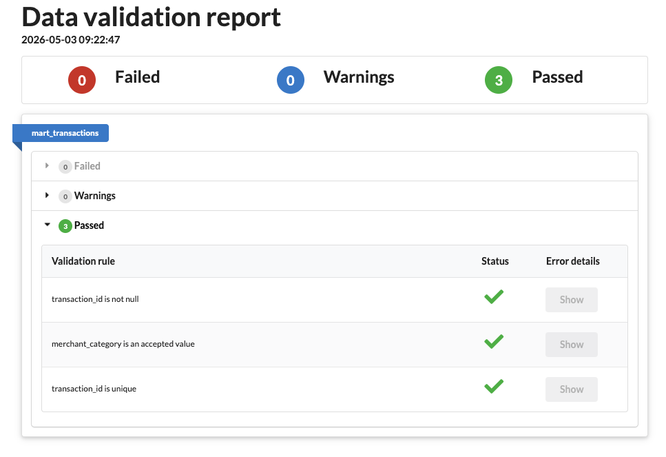Successful {targets} + {data.validator} run

otherwise a failure is reported

Errored {targets} + {data.validator} run

and clicking on ‘Show’ opens a table of the offending results.

Top of this section | ⬆️ Table of Contents

Analysis

What’s the point of organising this data if we’re not going to do something with it? This is where I start to really wonder if {targets} maybe has a bigger picture in mind when it connects up the data, because while dbt will do all of the processing in SQL, R will happily continue to do the analysis.

I think this is where a separation of concerns becomes necessary, and that depends on the scale of the data involved. While you or I working on a small project might be very happy to tie the analysis into the data preparation all in one place, Netflix probably wants to segregate the data processing and analysis steps into entirely different divisions, so tying a bow on the cleaned data and letting analysts pick it up from a database makes a lot more sense.

For my example, let’s say I’m interested in analysing which categories have out of the ordinary amounts of spend in a given month - have I spent more on groceries this month? To do that, I want to calculate the average spend in each category each month plus the variation and identify when the spend is more than a standard deviation away from the average.

Given that this needs the ‘final’ tables, it belongs in the models/marts folder. There is an analysis/ folder in the dbt project by default, but that’s for ad-hoc SQL queries that need to use ref() but don’t necessarily produce anything one wishes to persist.

Calculating the standard deviations relies on DuckDB’s helpers, which I don’t even want to consider writing in bare SQL myself. In models/mart/mart_category_outliers.sql:

with monthly as (
    select * from {{ ref('mart_category_trends') }}
),

stats as (
    select
        merchant_category,
        avg(total_aud)                                    as mean_spend,
        stddev_samp(total_aud)                            as sd_spend,
        count(*)                                          as n_months
    from monthly
    where total_aud > 0
    group by 1
    having count(*) > 1  -- need >1 observation for stddev
),

outliers as (
    select
        m.month,
        m.merchant_category,
        m.total_aud,
        s.mean_spend,
        m.total_aud - s.mean_spend                       as deviation,
        (m.total_aud - s.mean_spend) / s.sd_spend        as z_score
    from monthly m
    inner join stats s using (merchant_category)
    where m.total_aud > 0
      and abs((m.total_aud - s.mean_spend) / s.sd_spend) > 1
)

select * from outliers
order by abs(z_score) desc

This creates a new table in the database with the results.

The sd() function in R is no stranger to anyone who’s done stats, and it drops into this code cleanly because {dplyr} translates SQL, and supports DuckDB

monthly_outliers <- function(mart_monthly) {
  spend <- mart_monthly |>
    filter(total_spend_aud > 0)

  stats <- spend |>
    group_by(merchant_category) |>
    summarise(
      mean_spend = mean(total_spend_aud),
      sd_spend = sd(total_spend_aud),
      n_months = n(),
      .groups = "drop"
    ) |>
    filter(n_months > 1) # need >1 observation for sd

  spend |>
    inner_join(stats, by = "merchant_category") |>
    mutate(
      z_score = (total_spend_aud - mean_spend) / sd_spend,
      deviation = total_spend_aud - mean_spend
    ) |>
    filter(abs(z_score) > 1) |>
    arrange(desc(abs(z_score))) |>
    select(
      month,
      merchant_category,
      total_spend_aud,
      mean_spend,
      deviation,
      z_score
    )
}

which one can examine by asking {dbplyr} to explain how it’s working

dplyr::copy_to(
  DBI::dbConnect(duckdb::duckdb()), 
  data.frame(x = c(2, 3, 1, 5, 4)), 
  "example"
) |> 
  dplyr::summarise(sd_x = sd(x, na.rm = TRUE)) |>
  dplyr::show_query()

## <SQL>
## SELECT STDDEV(x) AS sd_x
## FROM example

which shows that it uses the alias STDDEV(x).

Top of this section | ⬆️ Table of Contents

The Complete Workflow

That’s all the pieces I need to push data in the exported CSVs through the pipe and produce a database of monthly aggregated, categorised totals. Here’s how it looks in terms of the two tools.

The file structure is perhaps best seen in the docs website (see the next section), but essentially the files in models define the workflow

models
├── intermediate
│   ├── int_monthly_balances.sql
│   └── int_transactions_categorised.sql
├── marts
│   ├── mart_category_outliers.sql
│   ├── mart_category_trends.sql
│   ├── mart_transactions.sql
│   └── schema.yml
└── staging
    ├── sources.yml
    ├── stg_bank.sql
    ├── stg_cc.sql
    └── stg_transactions.sql

Throughout the dbt steps I’ve detailed here, each .sql model produced a corresponding table in the DuckDB database. Running

uv run dbt build

runs through the DAG identifying what needs to be run before what, then runs all the steps in order. An example of this running well looks like

01:51:09  Found 1 seed, 8 models, 4 data tests, 2 sources, 591 macros
01:51:09  
01:51:09  Concurrency: 1 threads (target='dev')
01:51:09  
01:51:09  1 of 13 START sql view model main.stg_bank ..................................... [RUN]
01:51:09  1 of 13 OK created sql view model main.stg_bank ................................ [OK in 0.04s]
01:51:09  2 of 13 START sql view model main.stg_cc ....................................... [RUN]
01:51:09  2 of 13 OK created sql view model main.stg_cc .................................. [OK in 0.02s]
01:51:09  3 of 13 START seed file main.seed_merchants .................................... [RUN]
01:51:09  3 of 13 OK loaded seed file main.seed_merchants ................................ [INSERT 402 in 0.02s]
01:51:09  4 of 13 START sql view model main.stg_transactions ............................. [RUN]
01:51:09  4 of 13 OK created sql view model main.stg_transactions ........................ [OK in 0.04s]
01:51:09  5 of 13 START sql view model main.int_transactions_categorised ................. [RUN]
01:51:09  5 of 13 OK created sql view model main.int_transactions_categorised ............ [OK in 0.03s]
01:51:09  6 of 13 START sql view model main.int_monthly_balances ......................... [RUN]
01:51:09  6 of 13 OK created sql view model main.int_monthly_balances .................... [OK in 0.03s]
01:51:09  7 of 13 START sql table model main.mart_category_trends ........................ [RUN]
01:51:09  7 of 13 OK created sql table model main.mart_category_trends ................... [OK in 0.22s]
01:51:09  8 of 13 START sql incremental model main.mart_transactions ..................... [RUN]
01:51:09  8 of 13 OK created sql incremental model main.mart_transactions ................ [OK in 0.26s]
01:51:09  9 of 13 START sql table model main.mart_category_outliers ...................... [RUN]
01:51:09  9 of 13 OK created sql table model main.mart_category_outliers ................. [OK in 0.01s]
01:51:09  10 of 13 START test assert_all_transactions_categorised ........................ [RUN]
01:51:09  10 of 13 WARN 34 assert_all_transactions_categorised ........................... [WARN 34 in 0.01s]
01:51:09  11 of 13 START test merchant_category_is_valid ................................. [RUN]
01:51:09  11 of 13 PASS merchant_category_is_valid ....................................... [PASS in 0.01s]
01:51:09  12 of 13 START test not_null_mart_transactions_transaction_id .................. [RUN]
01:51:09  12 of 13 PASS not_null_mart_transactions_transaction_id ........................ [PASS in 0.01s]
01:51:09  13 of 13 START test unique_mart_transactions_transaction_id .................... [RUN]
01:51:09  13 of 13 PASS unique_mart_transactions_transaction_id .......................... [PASS in 0.01s]
01:51:09  
01:51:09  Finished running 1 incremental model, 1 seed, 2 table models, 4 data tests, 5 view models in 0 hours 0 minutes and 0.78 seconds (0.78s).
01:51:09  
01:51:09  Completed with 1 warning:
01:51:09  
01:51:09  Warning in test assert_all_transactions_categorised (tests/assert_all_transactions_categorised.sql)
01:51:09  Got 34 results, configured to warn if != 0
01:51:09  
01:51:09    compiled code at target/compiled/slowbooks/tests/assert_all_transactions_categorised.sql
01:51:09  
01:51:09  Done. PASS=12 WARN=1 ERROR=0 SKIP=0 NO-OP=0 TOTAL=13

The times on the left side are in UTC, and I can’t find a way to change that, which may be for the best - one can always convert to local after the fact if needed.

Everything completed with an OK status except for the assertion which I’ve allowed to WARN because I haven’t categorised a handful of records.

Looking at the resulting database, e.g. in a terminal, shows all the tables which have been created

duckdb slowbooks.duckdb

DuckDB v1.5.2 (Variegata)
Enter ".help" for usage hints.
slowbooks D show tables;
┌──────────────────────────────┐
│             name             │
│           varchar            │
├──────────────────────────────┤
│ int_monthly_balances         │
│ int_transactions_categorised │
│ mart_category_outliers       │
│ mart_category_trends         │
│ mart_transactions            │
│ seed_merchants               │
│ stg_bank                     │
│ stg_cc                       │
│ stg_transactions             │
└──────────────────────────────┘

The {targets} workflow is defined as a list within the _targets.R file

list(
  # format="file" means targets re-runs downstream when file list or contents change
  tar_target(
    cc_files,
    cc_list,
    format = "file"
  ),
  tar_target(
    bank_files,
    bank_list,
    format = "file"
  ),
  tar_target(merchant_file, "../seeds/seed_merchants.csv", format = "file"),

  # Seeds
  tar_target(merchants, readr::read_csv(merchant_file, show_col_types = FALSE)),

  # Staging — passing file vectors directly so targets tracks dependencies correctly
  tar_target(stg_bank, stage_source(bank_files)),
  tar_target(stg_cc, stage_source(cc_files)),
  tar_target(stg_txns, stg_transactions(stg_bank, stg_cc)),

  # Intermediate
  tar_target(int_categorised, categorise_transactions(stg_txns, merchants)),
  tar_target(int_monthly, monthly_balances(int_categorised)),

  # Tests
  tar_target(validation, run_tests(int_categorised)),
  tar_target(is_violation, validation_violation(validation)),

  # Marts
  tar_target(mart_txns, mart_transactions(int_categorised)),
  tar_target(mart_monthly, mart_monthly_summary(mart_txns)),

  # Persist to DuckDB
  tar_target(
    db_mart_transactions,
    write_to_duckdb(mart_txns, "mart_transactions")
  ),
  tar_target(
    db_mart_monthly_summary,
    write_to_duckdb(mart_monthly, "mart_monthly_summary")
  ),

  # Analysis
  tar_target(outliers, monthly_outliers(mart_monthly))
)

and running tar_make() (or with the added validation, tar_make_catch()) from the working directory containing that file, the workflow is run

+ bank_files dispatched                      
✔ bank_files completed [281ms, 74.42 kB]
+ cc_files dispatched
✔ cc_files completed [0ms, 137.82 kB]
+ merchant_file dispatched
✔ merchant_file completed [1ms, 15.89 kB]
+ stg_bank dispatched
✔ stg_bank completed [88ms, 12.98 kB]
+ stg_cc dispatched
✔ stg_cc completed [84ms, 18.60 kB]
+ merchants dispatched
✔ merchants completed [137ms, 7.33 kB]
+ stg_txns dispatched
✔ stg_txns completed [101ms, 71.10 kB]
+ int_categorised dispatched
✔ int_categorised completed [871ms, 86.06 kB]                
+ mart_txns dispatched                                       
✔ mart_txns completed [0ms, 86.06 kB]                        
+ validation dispatched                                      
✔ validation completed [2.7s, 5.10 kB]                        
+ int_monthly dispatched                                      
✔ int_monthly completed [3ms, 650 B]                          
+ mart_monthly dispatched                                     
✔ mart_monthly completed [4ms, 2.78 kB]                       
+ db_mart_transactions dispatched                             
✔ db_mart_transactions completed [83ms, 70 B]                 
+ is_violation dispatched                                     
✔ is_violation completed [1ms, 48 B]                          
+ db_mart_monthly_summary dispatched                          
✔ db_mart_monthly_summary completed [79ms, 72 B]              
+ outliers dispatched                                         
✔ outliers completed [10ms, 2.30 kB]                          
✔ ended pipeline [4.6s, 16 completed, 0 skipped]

An important difference is that writing to the database only happened in two of the steps at the end, so the (distinct) database only contains those tables

duckdb targets/slowbooks_r.duckdb

DuckDB v1.5.2 (Variegata)
Enter ".help" for usage hints.
slowbooks_r D show tables;
┌──────────────────────┐
│         name         │
│       varchar        │
├──────────────────────┤
│ mart_monthly_summary │
│ mart_transactions    │
└──────────────────────┘

There’s nothing stopping me from also adding a write_to_duckdb() (a function which just opens the database, writes a table, then closes) call for any of the other steps, but I was satisfied that I am building the same thing in both cases.

Top of this section | ⬆️ Table of Contents

DAG / Visualisation / Docs

The similarity to a Makefile of these approaches depends on being able to determine what has ‘changed’ and what is the same, and this is where the two approaches differ. Both consider the workflow as a Directed Acyclic Graph (DAG) with steps taking dependencies on previous steps or data sources. This means I can visualise the workflow as a graph, but also makes for some important differences between how things actually run.

Every time I run dbt build the entire model is re-run. If the model is ‘incremental’ then it won’t need to do a full CREATE TABLE or re-categorise existing records every time, but all of the steps will be re-run. This also makes for more complexity if I do want to re-categorise existing records, in which case I need to add --full-refresh to the build step.

With the model defined I can visualise it by generating and serving the documentation site with
```
uv run dbt docs generate && uv run dbt docs serve 
```
This builds a site locally hosted which includes all of the SQL code and a lineage graph showing how different pieces connect together

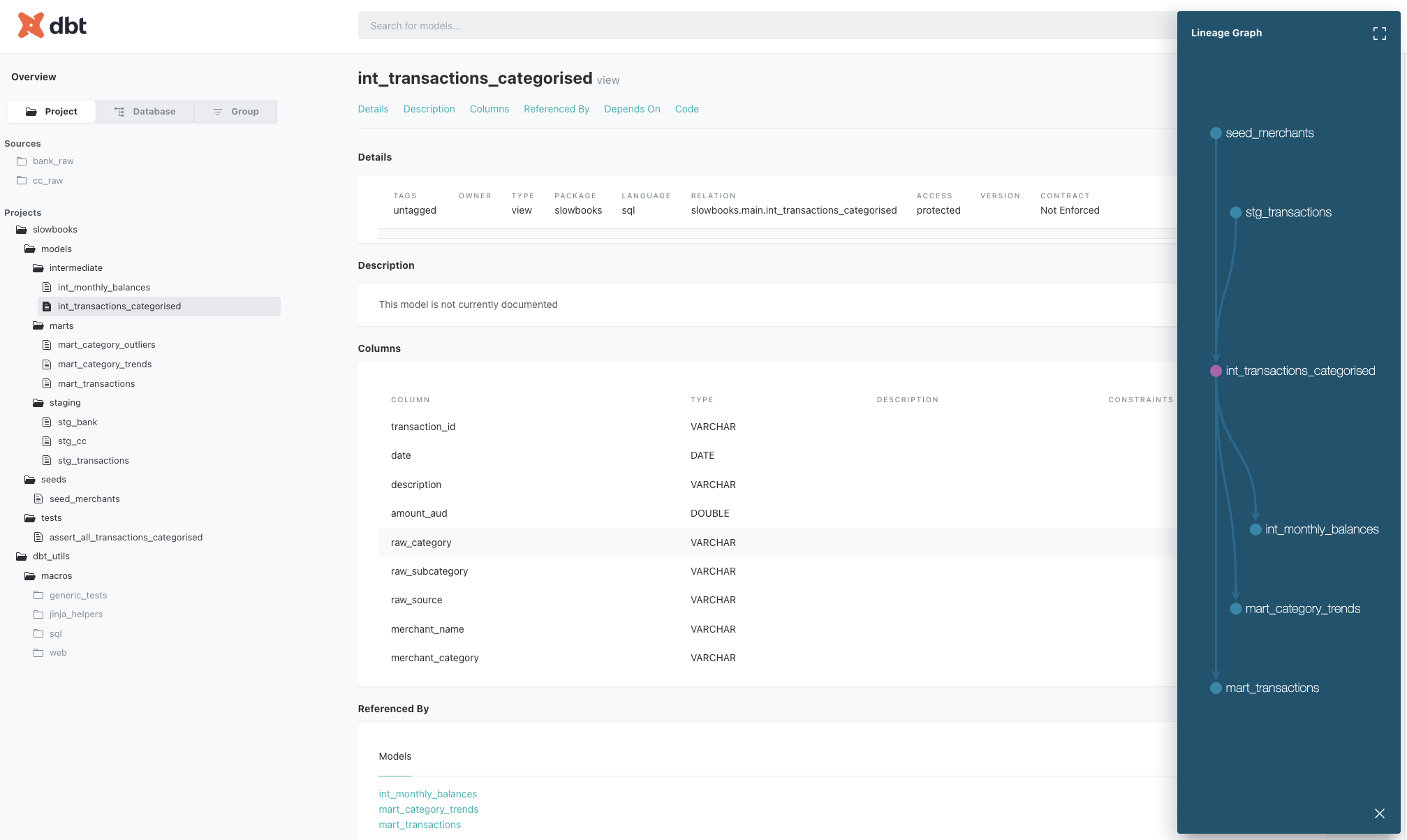dbt docs site (click to embiggen)

Expanding this pane shows more of the DAG for the project, though not all of the connections

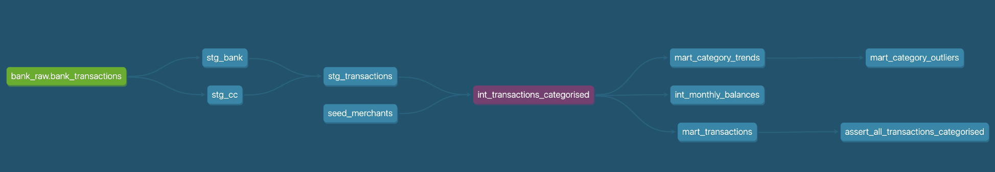dbt DAG for the whole slowbooks project (click to embiggen)

This is really nice, and shows how the data flows from the raw data to the final summary.
This is where I think {targets} may have an advantage over dbt – since the workflow considers a hash of the data objects to determine what has changed, even if the code remains the same, it can identify which steps of the DAG are invalidated, and can skip over any steps which don’t need to be re-run.

This is significant when the data you’re processing is no longer necessarily local to the machine running the pipeline. dbt performs the queries with SQL on the database (in this example the tables are written in DuckDB and materialised as views for downstream models), while the structure I’m using for {targets} here explicitly pulls in the data for R-native processing. I could make it more remote and use lazy tbl() operations via {dbplyr}, but it’s a trade-off one needs to consider.

A full DAG for the project can be produced in an editor able to render HTML such as RStudio or Positron, with
```
targets::tar_visnetwork()
```
producing an interactive plot

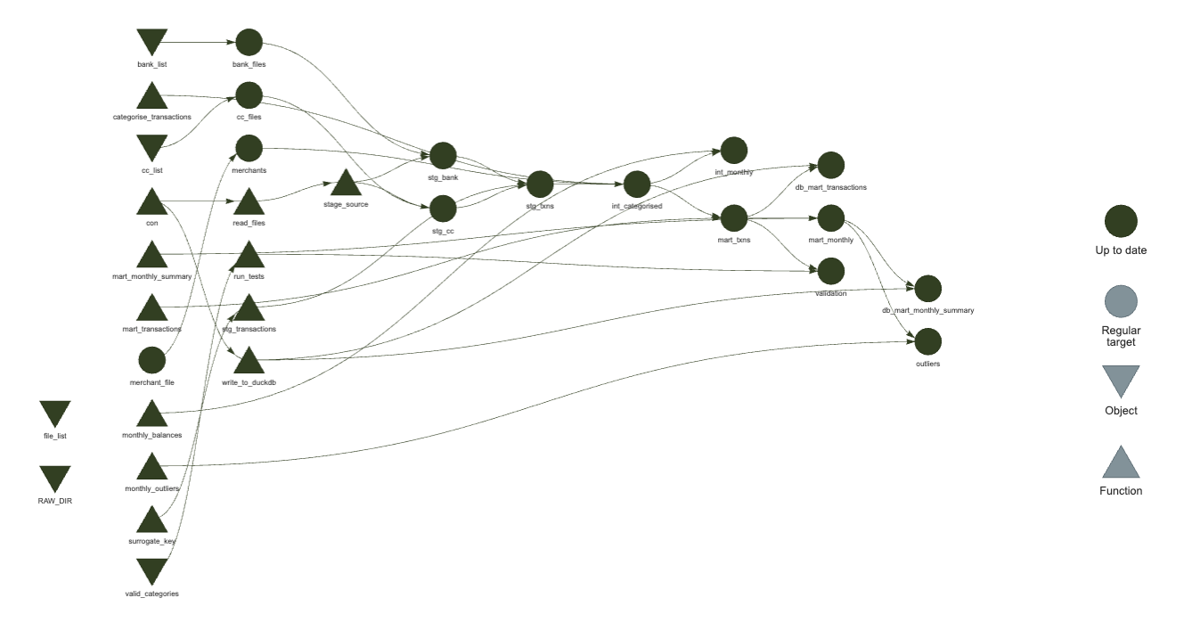Up-to-date {targets} DAG visualisation (click to embiggen)

If I change some of the code in the mart definition, and re-evaluate just that function, then re-running targets::tar_visnetwork() shows me which nodes are affected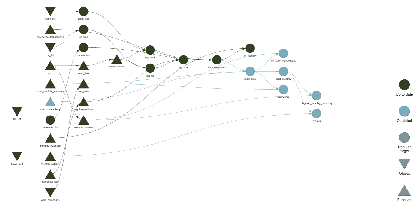

Invalidated {targets} DAG visualisation (click to embiggen)

(note the different colour of some nodes). This is fantastic!

What’s more, if I have a failing test during the validation, I can see what is downstream from that

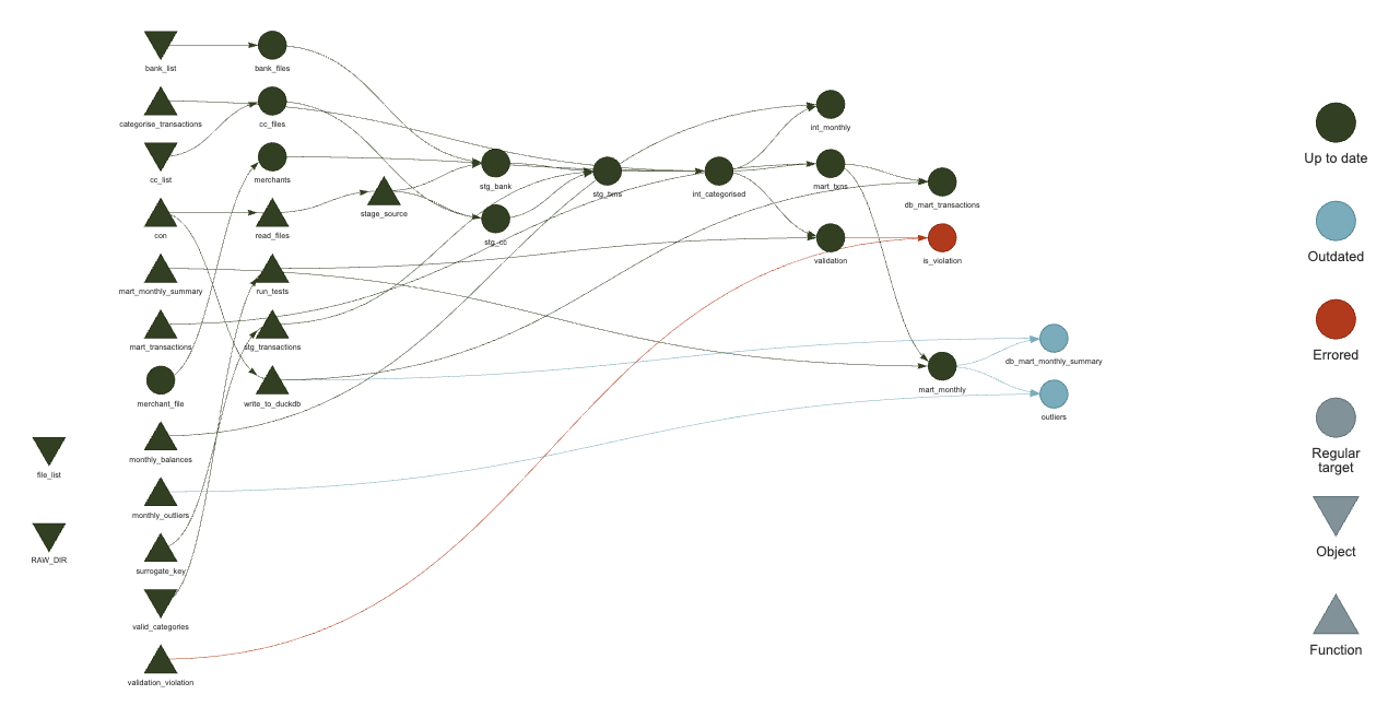Failed validation in {targets} DAG (click to embiggen)

That did require following the article in the {data.validator} docs to define
```
validation_violation <- function(report) {
  violations_exist <- report$get_validations() %>%
    summarise(
      sum(num.violations, na.rm = TRUE) > 0
    ) %>%
    pull()
  if (isTRUE(violations_exist)) {
    rlang::abort(
      "Validation schema error",
      body = capture.output(report),
      class = "validation_violation"
    )
  }
  FALSE
}
```
and adding to the target
```
tar_target(is_violation, validation_violation(validation)),
```
and instead of running tar_make(), using a tryCatch()
```
tar_make_catch <- function() {
    tryCatch(
        tar_make(),
        validation_violation = function(e) {
            print(e)
            tar_visnetwork()
        }
    )
}
```
Incredibly powerful stuff, right?

Top of this section | ⬆️ Table of Contents

Exploration

I only built the exploration dashboard as part of the dbt project because I’ve built plenty of shiny apps - I wanted to see what Claude could build based on this database data source. It built a streamlit app which shows the monthly spend broken down by category, and I had it add filters for the various categories, tables of transactions, and the monthly outliers.

The dashboard works great, albeit not perfectly. It looks something like this

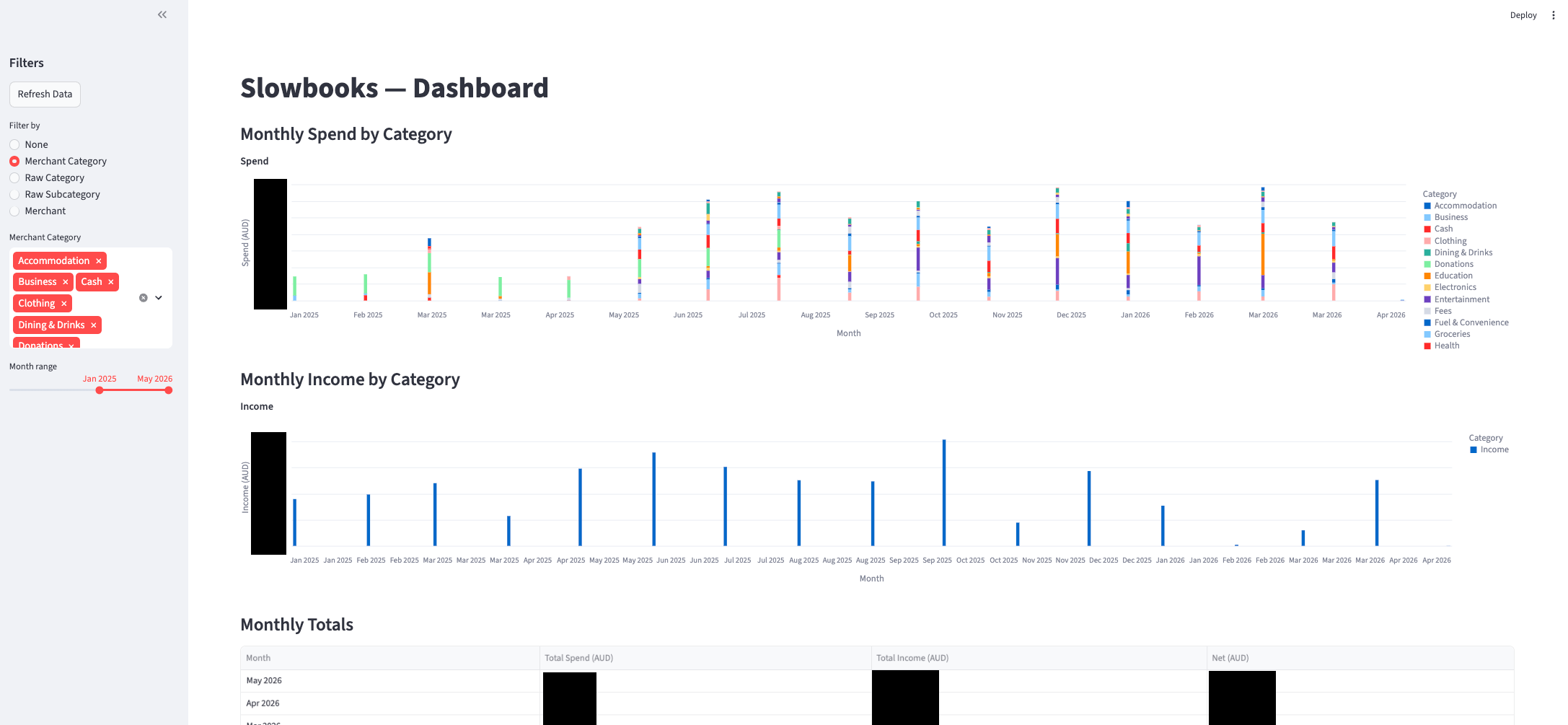
Slowbooks dashboard (click to embiggen)

There’s obvious issues with it - not least that the legend is incomplete, but for the sort of exploration I wanted to try out, it’s a great starting point.

It reads the summary tables directly from the database, so the analysis doesn’t need to happen within the app – a nice separation of business logic and visualisation.

Comparison

As a final sanity check, I’ll confirm that I get the same number of transactions in the monthly trend tables which are saved to both databases, albeit with different names

duckdb slowbooks.duckdb -c "select sum(transaction_count) from mart_category_trends;"
┌────────────────────────┐
│ sum(transaction_count) │
│         int128         │
├────────────────────────┤
│                   2028 │
└────────────────────────┘

duckdb targets/slowbooks_r.duckdb -c "select sum(transaction_count) from mart_monthly_summary;"
┌────────────────────────┐
│ sum(transaction_count) │
│         int128         │
├────────────────────────┤
│                   2028 │
└────────────────────────┘

🎉

As for what I like and don’t like about each approach:

Language: I don’t reach for SQL as a primary language (it’s absolutely the second language everyone who codes with data should learn, in my opinion) so having to write everything in SQL myself doesn’t appeal so much to me. I’m very happy to be able to use {dplyr} more or less everywhere and have it write the SQL for me. On the other hand, I can see the value in moving to a language that’s closer to the data itself – the abstractions change over time ({dplyr} is notorious for this) so with fewer bells and whistles likely comes more stability. Provided the helper functions are available for things like basic statistics (e.g. in DuckDB) this doesn’t sound like too much of a downside. Doing a bit more research, it seems that dbt does support using Python for models, provided the adapter supports it (which dbt-duckdb does), so that’s a big win for those more familiar with Python, although I am under the impression that not everything works exactly the same for these models.
Connection: I appreciate the massive leg-up that dbt offers in terms of handling connections to sources via extensions (e.g. dbt-duckdb). I’m sure if you’re not used to that then it looks like magic, but those familiar with working with databases via {dbplyr} and {DBI} it loses some of the wonder. Importantly, the dbt SQL code all runs within the database - downstream models rely on views so the data never really leaves the database. The R version could get closer to this, but I suspect the more common use-case is to actually pull down all of the data in which case it’s likely to fit within RAM.
Version Control: For people not used to committing their work, again this seems like a huge step up, but R users get taught fairly early on to work with git and track their code, even if it’s just scripts. Someone used to just throwing SQL at a database from a terminal might be rightly amazed at the benefits opened up by tracking code this way, but for me it’s the default state.
Layout: dbt has so many files for even a simple project that my VSCode file explorer runs off the screen. {targets} has everything in a single file. This could be organised more like dbt with a liberal use of source() calls at the top of _targets.R, say for each model and some utils.
Interrogation: Perhaps there’s some more tooling I’m not aware of, but the {targets} visualisation of the DAG is a clear winner for me. Part of the tradeoff between ‘run everything locally’ and ‘run everything remotely’ is that I can inspect the intermediate data in the {targets} workflow with tar_read(id) and see what’s happening. I can read the generated table in the database, but for smallish data being able to just crack it open and have a look wins for me.

Conclusion

I’ve vastly grown my understanding of both dbt and {targets} and have a much greater appreciation for what goes into using each of these to move and curate data. Plus, now I have a cool new toy I’ve built to explore my finances. I’m not sharing the code itself – partly so that I don’t risk committing my own finance data by accident, and partly because what I’ve done here isn’t anything you need to build on; if you’re interested in learning either or both of these tools, I recommend you do what I did and build a toy project.

I’m interested to hear what you think of this comparison – have I overlooked some significant difference or similarity? Some use-case where one of them would really shine over the other? Have I misrepresented something? I’m here to learn, so by all means please do let me know. And if you’re looking for someone with a history of programming and data who digs into projects this way, I’m on the market for opportunities.

As always, I can be found on Mastodon and the comment section below.

devtools::session_info()

## ─ Session info ───────────────────────────────────────────────────────────────
##  setting  value
##  version  R version 4.5.3 (2026-03-11)
##  os       macOS Tahoe 26.3.1
##  system   aarch64, darwin20
##  ui       X11
##  language (EN)
##  collate  en_US.UTF-8
##  ctype    en_US.UTF-8
##  tz       Australia/Adelaide
##  date     2026-05-04
##  pandoc   3.6.3 @ /Applications/RStudio.app/Contents/Resources/app/quarto/bin/tools/aarch64/ (via rmarkdown)
##  quarto   1.7.31 @ /usr/local/bin/quarto
## 
## ─ Packages ───────────────────────────────────────────────────────────────────
##  package     * version date (UTC) lib source
##  blob          1.3.0   2026-01-14 [1] CRAN (R 4.5.2)
##  blogdown      1.23    2026-01-18 [1] CRAN (R 4.5.2)
##  bookdown      0.46    2025-12-05 [1] CRAN (R 4.5.2)
##  bslib         0.10.0  2026-01-26 [1] CRAN (R 4.5.2)
##  cachem        1.1.0   2024-05-16 [1] CRAN (R 4.5.0)
##  cli           3.6.5   2025-04-23 [1] CRAN (R 4.5.0)
##  DBI           1.3.0   2026-02-25 [1] CRAN (R 4.5.2)
##  dbplyr        2.5.2   2026-02-13 [1] CRAN (R 4.5.2)
##  devtools      2.4.6   2025-10-03 [1] CRAN (R 4.5.0)
##  digest        0.6.39  2025-11-19 [1] CRAN (R 4.5.2)
##  dplyr         1.2.1   2026-04-03 [1] CRAN (R 4.5.2)
##  duckdb        1.5.2   2026-04-13 [1] CRAN (R 4.5.2)
##  ellipsis      0.3.2   2021-04-29 [1] CRAN (R 4.5.0)
##  evaluate      1.0.5   2025-08-27 [1] CRAN (R 4.5.0)
##  fastmap       1.2.0   2024-05-15 [1] CRAN (R 4.5.0)
##  fs            1.6.7   2026-03-06 [1] CRAN (R 4.5.2)
##  generics      0.1.4   2025-05-09 [1] CRAN (R 4.5.0)
##  glue          1.8.1   2026-04-17 [1] CRAN (R 4.5.2)
##  htmltools     0.5.9   2025-12-04 [1] CRAN (R 4.5.2)
##  jquerylib     0.1.4   2021-04-26 [1] CRAN (R 4.5.0)
##  jsonlite      2.0.0   2025-03-27 [1] CRAN (R 4.5.0)
##  knitr         1.51    2025-12-20 [1] CRAN (R 4.5.2)
##  lifecycle     1.0.5   2026-01-08 [1] CRAN (R 4.5.2)
##  magrittr      2.0.4   2025-09-12 [1] CRAN (R 4.5.0)
##  memoise       2.0.1   2021-11-26 [1] CRAN (R 4.5.0)
##  otel          0.2.0   2025-08-29 [1] CRAN (R 4.5.0)
##  pillar        1.11.1  2025-09-17 [1] CRAN (R 4.5.0)
##  pkgbuild      1.4.8   2025-05-26 [1] CRAN (R 4.5.0)
##  pkgconfig     2.0.3   2019-09-22 [1] CRAN (R 4.5.0)
##  pkgload       1.5.0   2026-02-03 [1] CRAN (R 4.5.2)
##  purrr         1.2.2   2026-04-10 [1] CRAN (R 4.5.2)
##  R6            2.6.1   2025-02-15 [1] CRAN (R 4.5.0)
##  remotes       2.5.0   2024-03-17 [1] CRAN (R 4.5.0)
##  rlang         1.1.7   2026-01-09 [1] CRAN (R 4.5.2)
##  rmarkdown     2.30    2025-09-28 [1] CRAN (R 4.5.0)
##  rstudioapi    0.18.0  2026-01-16 [1] CRAN (R 4.5.2)
##  sass          0.4.10  2025-04-11 [1] CRAN (R 4.5.0)
##  sessioninfo   1.2.3   2025-02-05 [1] CRAN (R 4.5.0)
##  tibble        3.3.1   2026-01-11 [1] CRAN (R 4.5.2)
##  tidyselect    1.2.1   2024-03-11 [1] CRAN (R 4.5.0)
##  usethis       3.2.1   2025-09-06 [1] CRAN (R 4.5.0)
##  vctrs         0.7.1   2026-01-23 [1] CRAN (R 4.5.2)
##  withr         3.0.2   2024-10-28 [1] CRAN (R 4.5.0)
##  xfun          0.56    2026-01-18 [1] CRAN (R 4.5.2)
##  yaml          2.3.12  2025-12-10 [1] CRAN (R 4.5.2)
## 
##  [1] /Library/Frameworks/R.framework/Versions/4.5-arm64/Resources/library
## 
## ──────────────────────────────────────────────────────────────────────────────

dbt rstats

Comparing R's {targets} and dbt for Data Engineering

dbt

{targets}

Comparing Workflows

Staging - Load Data

Intermediate - Joins and Enrichment

Marts - Summaries and Outputs

Tests / Validation

Analysis

The Complete Workflow

DAG / Visualisation / Docs

Exploration

Comparison

Other Solutions

Conclusion

See also